Scientific data is concerned with measuring and hence data, whether that is qualitative or quantitative. In pharmaceutical microbiology, this could be a number of cells or colony forming units, a series of growth or no growth results; and incidences of microorganisms. Gathering such data allows for trending and enables control to be achieved.
With microbial numbers, it is a regulatory expectation that alert and action levels be set. Alert and action levels are not specifications - they are ‘snap-shot’ indicators of potential adverse or upward trends, or out-of-control situations. Alert and action levels are used to detect shifts from the norm and to indicate if an individual result or process is potentially out-of-control. Therefore, what is important is the data pattern.
The standard approach is to set alert and action levels based on a set of historical data. Understanding past data enables for a more accurate assessment of current data in relation to the performance of a sample, system or environment. Furthermore, the use of this information ensures that the levels applied relate in some form to past data rather than being based on an arbitrary figure. Setting alert and action levels is hampered by data sets being distributed unusually, with the data containing many zeros (and so skewed to the left when a histogram is produced). This type of quality attribute is typically called a zero-inflated variable. Furthermore, there will often be occasional high values leading to a relatively high dispersal. The data is not always predictable and will contain a relatively high level of variability. One way to overcome this is through the use of the percentile cut-off approach.
To illustrate the percentile cut-off approach, a data set depicting Grade C surface data from a cleanroom has been used. Summarised in Table 1 is the data distribution, along with the same set of data trended in Figure 1.
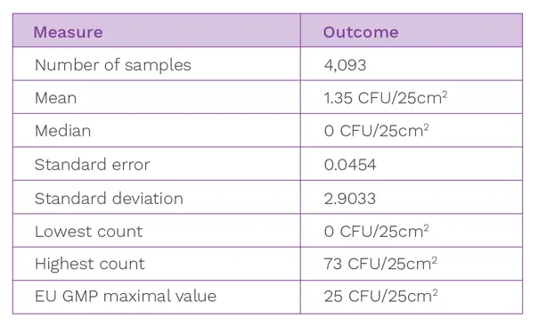
Table 1: Cleanroom data set summary
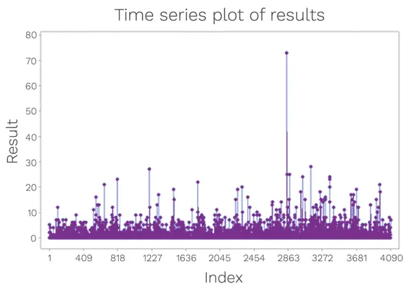
Figure 1: Data set from surface monitoring in a cleanroom
A consideration needs to be made as to whether any outliers will be removed from the data set. Outliers may be removed from calculations provided a justification is included and where a special or unusual cause can be ascribed to the result in a way that indicates that the result was not part of the norm. Example scenarios include:
The presence of outliers can be assessed using Grubbs’ Test. This test can be used to detect outliers in a univariate data set. The data set shown in Figure 2 is formed of a relatively close set of associated numbers, with only one evident outlier value. It is important to note that the Grubbs’ Test is an iterative test and after the outlier has been removed from the data set, the test is run successively until no further outliers are detected.
Whether outliers are removed or included requires a value judgement and the degree to which data might be distorted by an unrepresentative set of values.
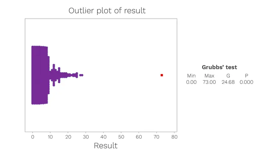
Figure 2: An examination of the Grade C surface data, to assess for outliers.
If that data conforms to normal distribution, then one approach that can be adopted for limit setting is to use the second and third standard deviations as the alert and action levels respectively. The standard deviation is the average amount of variability in the dataset. It then informs, on average, how far each value lies from the mean. This process is undertaken through the use of a histogram. In order to construct a histogram, the entire data set is required. The purpose of a histogram is to graphically summarise the distribution of a univariate data set. The histogram provides an indication of the centre (location) of the data, the spread (scale) of the data and any pattern of skewness of the data.
With the example data, a histogram has been constructed (Figure 3):
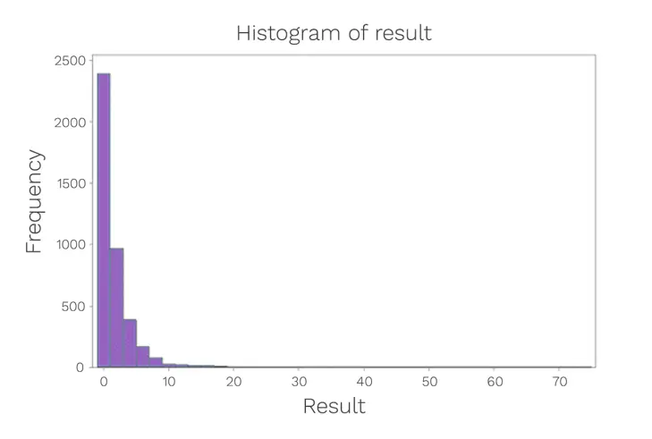
Figure 3: Data distribution histogram
When the data set is not naturally distributed, then an attempt can be made to convert the data to a pattern resembling normal distribution. One of the simplest ways to do so is via a power transformation. This can be used for values that are generally below 1000 which takes the square root and subjects this to the normal distribution plot. A power transformation is not always successful, especially in the case of extremely skewed data sets. In this case study, the data could not be transformed and therefore a different approach was adopted: The percentile cut-off approach.
A percentile is used in statistics to measure a value on a scale of one hundred that indicates the percent of a distribution that is equal to or below it For example, the 20th percentile is the value (or score) below which 20% of the observations may be found. The percentile usually indicates that a certain percentage falls below that percentile. For example, if we are interested in the 20th percentile, then 20% of values are below the number that the 20th percentile relates to.
However, if we want to know the percentile rank, then the application of the percentile is slightly different. Here, the nth percentile is the smallest score that is greater than or equal to a certain percentage of the scores. That is the percentage of data that falls at or below a certain observation.
For alert and action levels, it is customary to use the 95th percentile to assess the alert level and the 99th percentile to assess the action level. These percentiles work for Poisson-distributed data in terms of equivalence with the standard deviation approach. As indicated above, for normally distributed data, the alert is the mean plus 2x standard deviations (and this is equivalent to 95% probability) and the action level at mean plus 3x standard deviations (equivalent to 99.7% probability).
Using our existing data set, if we attempted to set alert and action levels using the 95th and 99th percentiles, this would lead to the following:
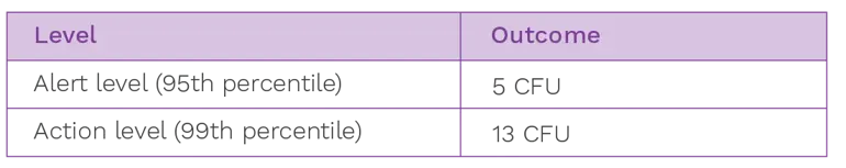
Table 2: Alert and action level table
It is always advisable to deploy professional judgement when reviewing alert and action levels and it may be that justified modifications need to be made. For example, with the upper level, any calculated level cannot exceed a specification (such as a limit published by a regulator).
With the lower level, should the data set be extremely good, caution is also required. For example, setting a Grade C contact plate alert level at 1 CFU/25cm2 might be unrealistically low in terms of being unrepresentative of what an area is capable of over the longer term. It may also be that reacting to a pattern of three 1 CFU creates a pattern of zero results which might not add value when performing an investigation. Furthermore, there are concerns about setting a limit so low in relation to possible errors arising from sampling or testing. Here the results obtained may be more prone to low level contamination arising from sampling or testing (again with a count of 1 CFU).
Alert levels should be set at the local plant level so that the data clearly relates to conditions under which specific pharmaceutical products are processed. This is important given variations in practice and geographically distinct microbiota. The approach for setting levels should be based on the distribution of the data and standard deviation should only be selected in cases where the data conforms to a normal distribution. Where it does not, alternative approaches need to be selected. A suitable tool for consideration is the percentile cut-off method (there are, of course, other approaches). Percentiles have the advantage of being resistant to outliers in the data set and less prone to other forms of variation, provided a sufficiently large data set is selected.
The frequency of reviewing will depend upon the amount of historical data and the criticality of the sample.

